scipy.stats.kappa4

scipy.stats.kappa4 = <scipy.stats._continuous_distns.kappa4_gen object>

Kappa 4 parameter distribution.

As an instance of the rv_continuous class, kappa4 object inherits from it a collection of generic methods (see below for the full list), and completes them with details specific for this particular distribution.

Notes

The probability density function for kappa4 is:

kappa4.pdf(x, h, k) = (1.0 - k*x)**(1.0/k - 1.0)*
                      (1.0 - h*(1.0 - k*x)**(1.0/k))**(1.0/h-1)

if h and k are not equal to 0.

If h or k are zero then the pdf can be simplified:

h = 0 and k != 0:

kappa4.pdf(x, h, k) = (1.0 - k*x)**(1.0/k - 1.0)*
                      exp(-(1.0 - k*x)**(1.0/k))

h != 0 and k = 0:

kappa4.pdf(x, h, k) = exp(-x)*(1.0 - h*exp(-x))**(1.0/h - 1.0)

h = 0 and k = 0:

kappa4.pdf(x, h, k) = exp(-x)*exp(-exp(-x))

kappa4 takes h and k as shape parameters.

The kappa4 distribution returns other distributions when certain h and k values are used.

h	k=0.0	k=1.0	-inf<=k<=inf
-1.0	Logistic logistic(x)		Generalized Logistic(1)
0.0	Gumbel gumbel_r(x)	Reverse Exponential(2)	Generalized Extreme Value genextreme(x, k)
1.0	Exponential expon(x)	Uniform uniform(x)	Generalized Pareto genpareto(x, -k)

1. There are at least five generalized logistic distributions. Four are described here: https://en.wikipedia.org/wiki/Generalized_logistic_distribution The “fifth” one is the one kappa4 should match which currently isn’t implemented in scipy: https://en.wikipedia.org/wiki/Talk:Generalized_logistic_distribution http://www.mathwave.com/help/easyfit/html/analyses/distributions/gen_logistic.html
2. This distribution is currently not in scipy.

References

J.C. Finney, “Optimization of a Skewed Logistic Distribution With Respect to the Kolmogorov-Smirnov Test”, A Dissertation Submitted to the Graduate Faculty of the Louisiana State University and Agricultural and Mechanical College, (August, 2004), http://etd.lsu.edu/docs/available/etd-05182004-144851/unrestricted/Finney_dis.pdf

J.R.M. Hosking, “The four-parameter kappa distribution”. IBM J. Res. Develop. 38 (3), 25 1-258 (1994).

B. Kumphon, A. Kaew-Man, P. Seenoi, “A Rainfall Distribution for the Lampao Site in the Chi River Basin, Thailand”, Journal of Water Resource and Protection, vol. 4, 866-869, (2012). http://file.scirp.org/pdf/JWARP20121000009_14676002.pdf

C. Winchester, “On Estimation of the Four-Parameter Kappa Distribution”, A Thesis Submitted to Dalhousie University, Halifax, Nova Scotia, (March 2000). http://www.nlc-bnc.ca/obj/s4/f2/dsk2/ftp01/MQ57336.pdf

The probability density above is defined in the “standardized” form. To shift and/or scale the distribution use the loc and scale parameters. Specifically, kappa4.pdf(x, h, k, loc, scale) is identically equivalent to kappa4.pdf(y, h, k) / scale with y = (x - loc) / scale.

Examples

>>> from scipy.stats import kappa4
>>> import matplotlib.pyplot as plt
>>> fig, ax = plt.subplots(1, 1)

Calculate a few first moments:

>>> h, k = 0.1, 0
>>> mean, var, skew, kurt = kappa4.stats(h, k, moments='mvsk')

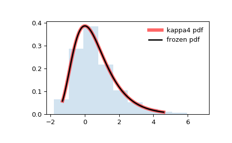
Display the probability density function (pdf):

>>> x = np.linspace(kappa4.ppf(0.01, h, k),
...                 kappa4.ppf(0.99, h, k), 100)
>>> ax.plot(x, kappa4.pdf(x, h, k),
...        'r-', lw=5, alpha=0.6, label='kappa4 pdf')

Alternatively, the distribution object can be called (as a function) to fix the shape, location and scale parameters. This returns a “frozen” RV object holding the given parameters fixed.

Freeze the distribution and display the frozen pdf:

>>> rv = kappa4(h, k)
>>> ax.plot(x, rv.pdf(x), 'k-', lw=2, label='frozen pdf')

Check accuracy of cdf and ppf:

>>> vals = kappa4.ppf([0.001, 0.5, 0.999], h, k)
>>> np.allclose([0.001, 0.5, 0.999], kappa4.cdf(vals, h, k))
True

Generate random numbers:

>>> r = kappa4.rvs(h, k, size=1000)

And compare the histogram:

>>> ax.hist(r, normed=True, histtype='stepfilled', alpha=0.2)
>>> ax.legend(loc='best', frameon=False)
>>> plt.show()

(Source code)

Methods

rvs(h, k, loc=0, scale=1, size=1, random_state=None)	Random variates.
pdf(x, h, k, loc=0, scale=1)	Probability density function.
logpdf(x, h, k, loc=0, scale=1)	Log of the probability density function.
cdf(x, h, k, loc=0, scale=1)	Cumulative distribution function.
logcdf(x, h, k, loc=0, scale=1)	Log of the cumulative distribution function.
sf(x, h, k, loc=0, scale=1)	Survival function (also defined as 1 - cdf, but sf is sometimes more accurate).
logsf(x, h, k, loc=0, scale=1)	Log of the survival function.
ppf(q, h, k, loc=0, scale=1)	Percent point function (inverse of cdf — percentiles).
isf(q, h, k, loc=0, scale=1)	Inverse survival function (inverse of sf).
moment(n, h, k, loc=0, scale=1)	Non-central moment of order n
stats(h, k, loc=0, scale=1, moments='mv')	Mean(‘m’), variance(‘v’), skew(‘s’), and/or kurtosis(‘k’).
entropy(h, k, loc=0, scale=1)	(Differential) entropy of the RV.
fit(data, h, k, loc=0, scale=1)	Parameter estimates for generic data.
expect(func, args=(h, k), loc=0, scale=1, lb=None, ub=None, conditional=False, **kwds)	Expected value of a function (of one argument) with respect to the distribution.
median(h, k, loc=0, scale=1)	Median of the distribution.
mean(h, k, loc=0, scale=1)	Mean of the distribution.
var(h, k, loc=0, scale=1)	Variance of the distribution.
std(h, k, loc=0, scale=1)	Standard deviation of the distribution.
interval(alpha, h, k, loc=0, scale=1)	Endpoints of the range that contains alpha percent of the distribution