scipy.signal.unit_impulse

scipy.signal.unit_impulse(shape, idx=None, dtype=<class 'float'>)

Unit impulse signal (discrete delta function) or unit basis vector.

Parameters:

shape : int or tuple of int

Number of samples in the output (1-D), or a tuple that represents the shape of the output (N-D).

idx : None or int or tuple of int or ‘mid’, optional

Index at which the value is 1. If None, defaults to the 0th element. If idx='mid', the impulse will be centered at shape // 2 in all dimensions. If an int, the impulse will be at idx in all dimensions.

dtype : data-type, optional

The desired data-type for the array, e.g., numpy.int8. Default is numpy.float64.

Returns:

y : ndarray

Output array containing an impulse signal.

Notes

The 1D case is also known as the Kronecker delta.

New in version 0.19.0.

Examples

An impulse at the 0th element (\(\delta[n]\)):

>>> from scipy import signal
>>> signal.unit_impulse(8)
array([ 1.,  0.,  0.,  0.,  0.,  0.,  0.,  0.])

Impulse offset by 2 samples (\(\delta[n-2]\)):

>>> signal.unit_impulse(7, 2)
array([ 0.,  0.,  1.,  0.,  0.,  0.,  0.])

2-dimensional impulse, centered:

>>> signal.unit_impulse((3, 3), 'mid')
array([[ 0.,  0.,  0.],
       [ 0.,  1.,  0.],
       [ 0.,  0.,  0.]])

Impulse at (2, 2), using broadcasting:

>>> signal.unit_impulse((4, 4), 2)
array([[ 0.,  0.,  0.,  0.],
       [ 0.,  0.,  0.,  0.],
       [ 0.,  0.,  1.,  0.],
       [ 0.,  0.,  0.,  0.]])

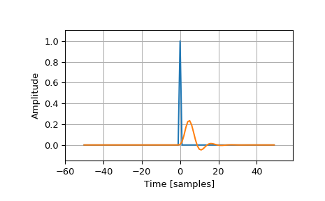
Plot the impulse response of a 4th-order Butterworth lowpass filter:

>>> imp = signal.unit_impulse(100, 'mid')
>>> b, a = signal.butter(4, 0.2)
>>> response = signal.lfilter(b, a, imp)

>>> import matplotlib.pyplot as plt
>>> plt.plot(np.arange(-50, 50), imp)
>>> plt.plot(np.arange(-50, 50), response)
>>> plt.margins(0.1, 0.1)
>>> plt.xlabel('Time [samples]')
>>> plt.ylabel('Amplitude')
>>> plt.grid(True)
>>> plt.show()

(Source code)