
scipy.signal.freqresp
-
scipy.signal.freqresp(system, w=None, n=10000)[source]¶ Calculate the frequency response of a continuous-time system.
Parameters: system : an instance of the
lticlass or a tuple describing the system.The following gives the number of elements in the tuple and the interpretation:
- 1 (instance of
lti) - 2 (num, den)
- 3 (zeros, poles, gain)
- 4 (A, B, C, D)
w : array_like, optional
Array of frequencies (in rad/s). Magnitude and phase data is calculated for every value in this array. If not given, a reasonable set will be calculated.
n : int, optional
Number of frequency points to compute if w is not given. The n frequencies are logarithmically spaced in an interval chosen to include the influence of the poles and zeros of the system.
Returns: w : 1D ndarray
Frequency array [rad/s]
H : 1D ndarray
Array of complex magnitude values
Notes
If (num, den) is passed in for
system, coefficients for both the numerator and denominator should be specified in descending exponent order (e.g.s^2 + 3s + 5would be represented as[1, 3, 5]).Examples
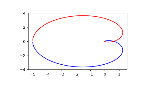
Generating the Nyquist plot of a transfer function
>>> from scipy import signal
>>> import matplotlib.pyplot as plt
Transfer function: H(s) = 5 / (s-1)^3
>>> s1 = signal.ZerosPolesGain([], [1, 1, 1], [5])
>>> w, H = signal.freqresp(s1)
>>> plt.figure()
>>> plt.plot(H.real, H.imag, "b")
>>> plt.plot(H.real, -H.imag, "r")
>>> plt.show()
- 1 (instance of